How to wrap text in Google Sheets

Wrapping text in Google Sheets is a useful method for formatting and organizing data and making it easier to read. It is a simple process that can be done in a few steps.

Here’s how to wrap text in Google Sheets.

Step 1: Open the Spreadsheet.

The first step is to open the spreadsheet that contains the text you wish to wrap. To do this, go to the Google Sheets homepage and click on the spreadsheet you wish to open.

Step 2: Select the Cells.

Once the spreadsheet is open, you need to select the cells where you want the text to wrap. To do this, click and drag your mouse to select the cells. You can also use the keyboard shortcut Ctrl+A to select all of the cells in the spreadsheet.

Step 3: Wrap Text.

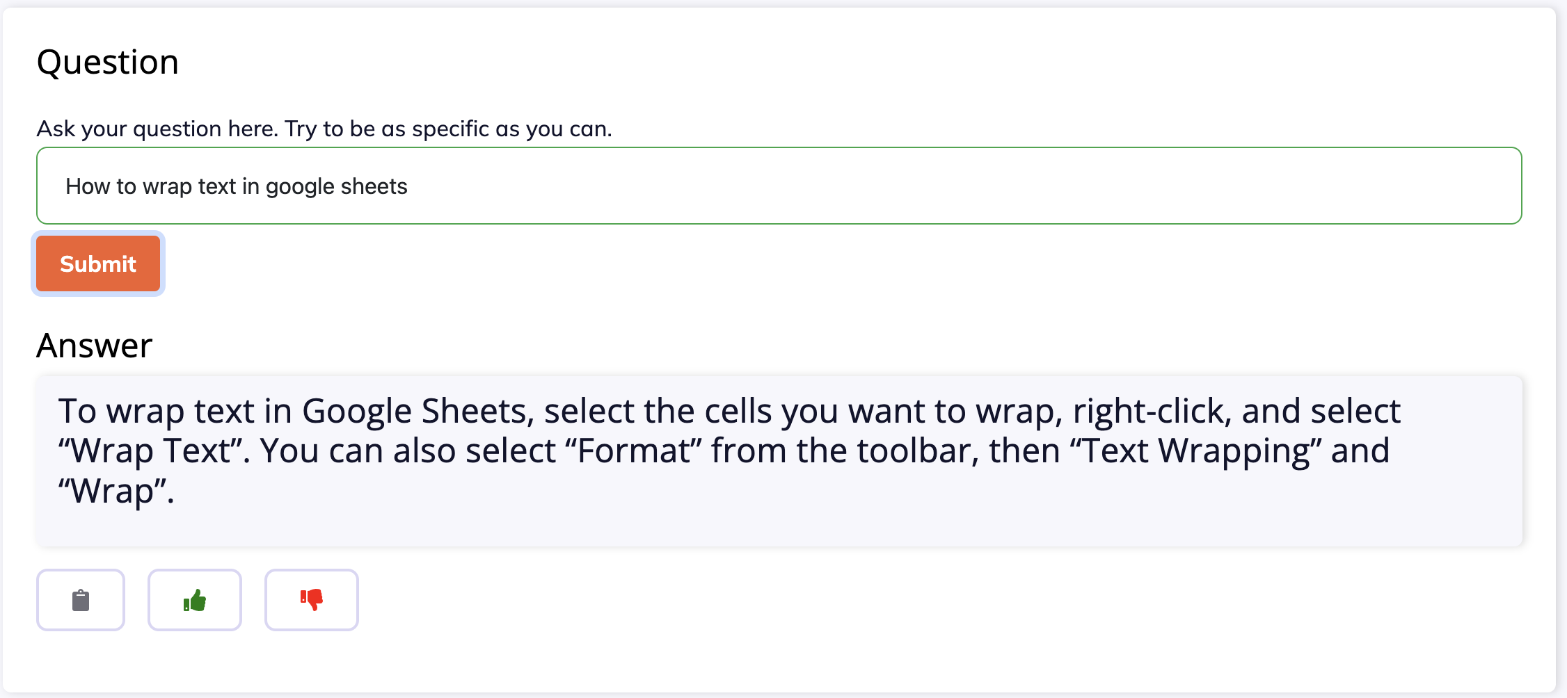
Once the cells are selected, you can wrap the text in the cells. To do this, click on the “Format” option in the top menu. Then, click on “Text Wrapping” and select the “Wrap” option. This will wrap the text in all of the selected cells.

Step 4: Adjust Cell Size.

Once you have wrapped the text, you may need to adjust the size of the cells to fit the wrapped text. To do this, click on the “Format” option in the top menu. Then, click on “Column Width” and adjust the size as necessary.

Step 5: Save the Spreadsheet.

Once you have finished wrapping the text, you need to save the spreadsheet. To do this, click on the “File” option in the top menu. Then, click on “Save” and enter a name for the file. This will save the file with the wrapped text.

Try asking similar questions from our AnswersBot powered by ChatGPT and instantly get step-by-step answers for Google Sheets. We’ve created a tool that makes it easier to generate formulas, Regex, and SQL from text descriptions.

Try FormulaGenerator today and make your spreadsheet work easier than ever.